We acquired four datasets for analyzing weather and event impacts on Manhattan subway ridership (2024-2025). This page documents both our data sources and the wrangling pipeline that transforms raw data into analysis-ready panels.

Part 1: Data Sources

MTA Subway Ridership

The Disaggregation Challenge:

The MTA ridership dataset is highly disaggregated to capture detailed fare collection patterns. Each hourly observation is broken down by:

11+ fare class categories: Full Fare, Senior/Disabled, Students (K-12 and college), Fair Fares (reduced-income riders), and various pass types (7-day, 30-day, unlimited)
2 payment methods: MetroCard (legacy magnetic stripe) and OMNY (contactless tap-to-pay)

This granularity creates a data explosion problem. For Manhattan’s 123 stations during a single week:

123 stations × 24 hours × 7 days × 11 fare categories × 2 payment methods = 227,304 records per week

For our complete 2024-2025 dataset (22 months ≈ 95 weeks), this would generate 21.6 million records—far exceeding the Socrata API’s 100,000-record pagination limit and creating unwieldy file sizes for analysis.

The Solution:

Since our research questions focus on total ridership rather than fare type breakdowns, we leveraged the Socrata API’s server-side aggregation capabilities. Using SUM() with $group, we aggregated across all fare types and payment methods before data transfer.

"$select" = "transit_timestamp, station_complex_id, station_complex,
             borough, SUM(ridership) as total_ridership",
"$group" = "transit_timestamp, station_complex_id, station_complex, borough"

This reduced records by 96% (from 21.6M to 1.92M), making monthly downloads feasible within API limits while preserving the station-hour granularity needed for our weather and event analyses.

This yielded 1,921,163 hourly observations across 123 Manhattan stations from 2024-01-01 to 2025-10-19.

# Daily trend (2024 only) with 7-day rolling average
daily_ridership <- ridership |>
  filter(year(date) == 2024) |>
  group_by(date) |>
  summarize(total = sum(total_ridership, na.rm = TRUE) / 1e6, .groups = "drop") |>
  arrange(date) |>
  mutate(
    rolling_avg = slide_dbl(total, mean, .before = 3, .after = 3, .complete = TRUE)
  )

p_daily <- daily_ridership |>
  ggplot(aes(x = date)) +
  geom_line(aes(y = total), color = okabe_ito$blue, alpha = 0.3, linewidth = 0.4) +
  geom_line(aes(y = rolling_avg), color = okabe_ito$blue, linewidth = 0.9) +
  scale_y_continuous(labels = comma) +
  labs(
    title = "Manhattan Subway Daily Ridership (2024)",
    subtitle = "7-day rolling average (bold) with daily values (faded)",
    x = NULL, y = "Daily Ridership (M)"
  ) +
  theme(plot.title = element_text(size = 11), plot.subtitle = element_text(size = 9))

# Hourly pattern
p_hourly <- ridership |>
  mutate(weekday_type = ifelse(wday(date) %in% 2:6, "Weekday", "Weekend")) |>
  group_by(hour, weekday_type) |>
  summarize(avg = mean(total_ridership, na.rm = TRUE) / 1000, .groups = "drop") |>
  ggplot(aes(x = hour, y = avg, color = weekday_type)) +
  geom_line(linewidth = 1) +
  scale_color_manual(values = c("Weekday" = okabe_ito$blue, "Weekend" = okabe_ito$vermillion)) +
  labs(title = "Average Hourly Pattern", x = "Hour", y = "Avg Ridership (K)", color = NULL) +
  theme(legend.position = "top", plot.title = element_text(size = 11))

# Top stations
p_top <- ridership |>
  group_by(station_complex) |>
  summarize(total = sum(total_ridership, na.rm = TRUE) / 1e6, .groups = "drop") |>
  slice_max(total, n = 30) |>
  arrange(total) |>
  mutate(
    # Truncate station names at first '(' for cleaner display
    station_short = str_replace(station_complex, "\\s*\\(.*", ""),
    # Make names unique by adding row number suffix if duplicates exist
    station_short = make.unique(station_short, sep = " "),
    # Use factor with levels in current order to preserve sorting
    station_short = factor(station_short, levels = station_short)
  ) |>
  ggplot(aes(x = total, y = station_short)) +
  geom_col(fill = okabe_ito$green) +
  scale_x_continuous(labels = comma) +
  labs(title = "Top 30 Manhattan Stations", x = "Total Ridership (M)", y = NULL) +
  theme(plot.title = element_text(size = 11), axis.text.y = element_text(size = 8))

p_top | (p_daily / p_hourly)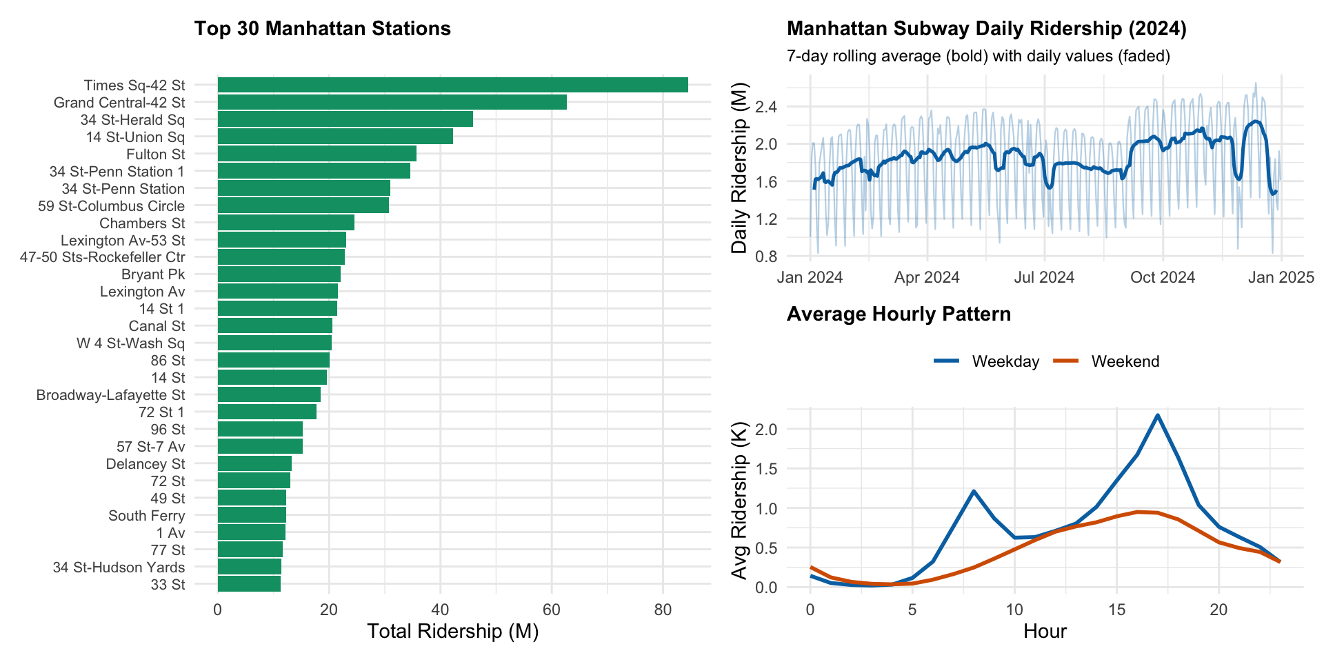

Key observations:

Daily trends show consistent ridership with clear weekly periodicity—weekday peaks and weekend dips. The 7-day rolling average smooths out day-to-day variation, revealing a stable baseline of ~2.5M daily rides.
Holiday dips are clearly visible, with ridership dropping sharply during July 4th, Thanksgiving, and Christmas/New Year periods—reflecting reduced commuter activity when offices close and residents leave the city.
Hourly patterns reveal the classic dual-peak commuter signature on weekdays (8-9 AM and 5-6 PM rush hours), while weekends show a single midday plateau reflecting leisure travel. Weekday ridership exceeds weekend by roughly 2x during peak hours.
Top stations are dominated by Midtown hubs (Penn Station, Times Square, Grand Central) that serve as major transit interchanges, followed by key employment centers and tourist destinations.

Download script: download_full_ridership_monthly.R

Weather Data

The NOAA API requires an authentication token, which we obtained from NOAA’s token request page. After receiving the token via email, we downloaded daily weather data for Central Park (located in Manhattan) covering 2020-2025. This provides consistent weather measurements applicable to all Manhattan stations.

weather <- read_csv('data/weather/central_park_weather_wide.csv', show_col_types = FALSE) |>
  mutate(date = as.Date(date))

The dataset contains 2,151 daily observations with max temperature, precipitation, and snowfall.

# Temperature and precipitation time series
p_ts <- weather |>
  filter(year(date) >= 2024) |>
  select(date, TMAX, PRCP) |>
  pivot_longer(cols = -date, names_to = "metric", values_to = "value") |>
  mutate(metric = ifelse(metric == "TMAX", "Max Temp (°F)", "Precipitation (in)")) |>
  ggplot(aes(x = date, y = value)) +
  geom_line(data = \(x) filter(x, metric == "Max Temp (°F)"), color = okabe_ito$vermillion, linewidth = 0.6) +
  geom_col(data = \(x) filter(x, metric == "Precipitation (in)"), fill = okabe_ito$sky_blue, alpha = 0.7) +
  facet_wrap(~metric, ncol = 1, scales = "free_y") +
  labs(title = "Central Park Weather (2024-2025)", x = NULL, y = NULL)

# Seasonal summary
weather_summary <- weather |>
  filter(year(date) >= 2024) |>
  mutate(
    season = case_when(
      month(date) %in% c(12, 1, 2) ~ "Winter",
      month(date) %in% c(3, 4, 5) ~ "Spring",
      month(date) %in% c(6, 7, 8) ~ "Summer",
      month(date) %in% c(9, 10, 11) ~ "Fall"
    ),
    season = factor(season, levels = c("Winter", "Spring", "Summer", "Fall")),
    month_abbr = month(date, label = TRUE, abbr = TRUE)
  )

# Seasonal aggregations
seasonal_weather <- weather_summary |>
  group_by(season) |>
  summarize(
    `Avg Temp (°F)` = mean(TMAX, na.rm = TRUE),
    `Storm Days (≥1in)` = sum(PRCP >= 1, na.rm = TRUE),
    `Heat Days (≥90°F)` = sum(TMAX >= 90, na.rm = TRUE),
    .groups = "drop"
  ) |>
  pivot_longer(cols = -season, names_to = "metric", values_to = "value")

# Plot seasonal summary
p_season <- seasonal_weather |>
  ggplot(aes(x = season, y = value)) +
  geom_col(aes(fill = season)) +
  scale_fill_manual(values = c(
    "Winter" = okabe_ito$sky_blue, "Spring" = okabe_ito$green,
    "Summer" = okabe_ito$orange, "Fall" = okabe_ito$pink
  )) +
  facet_wrap(~metric, scales = "free", ncol = 3) +
  labs(title = "Seasonal Weather Summary", x = NULL, y = NULL) +
  theme(legend.position = "none", axis.text.x = element_text(angle = 45, hjust = 1))

p_ts / p_season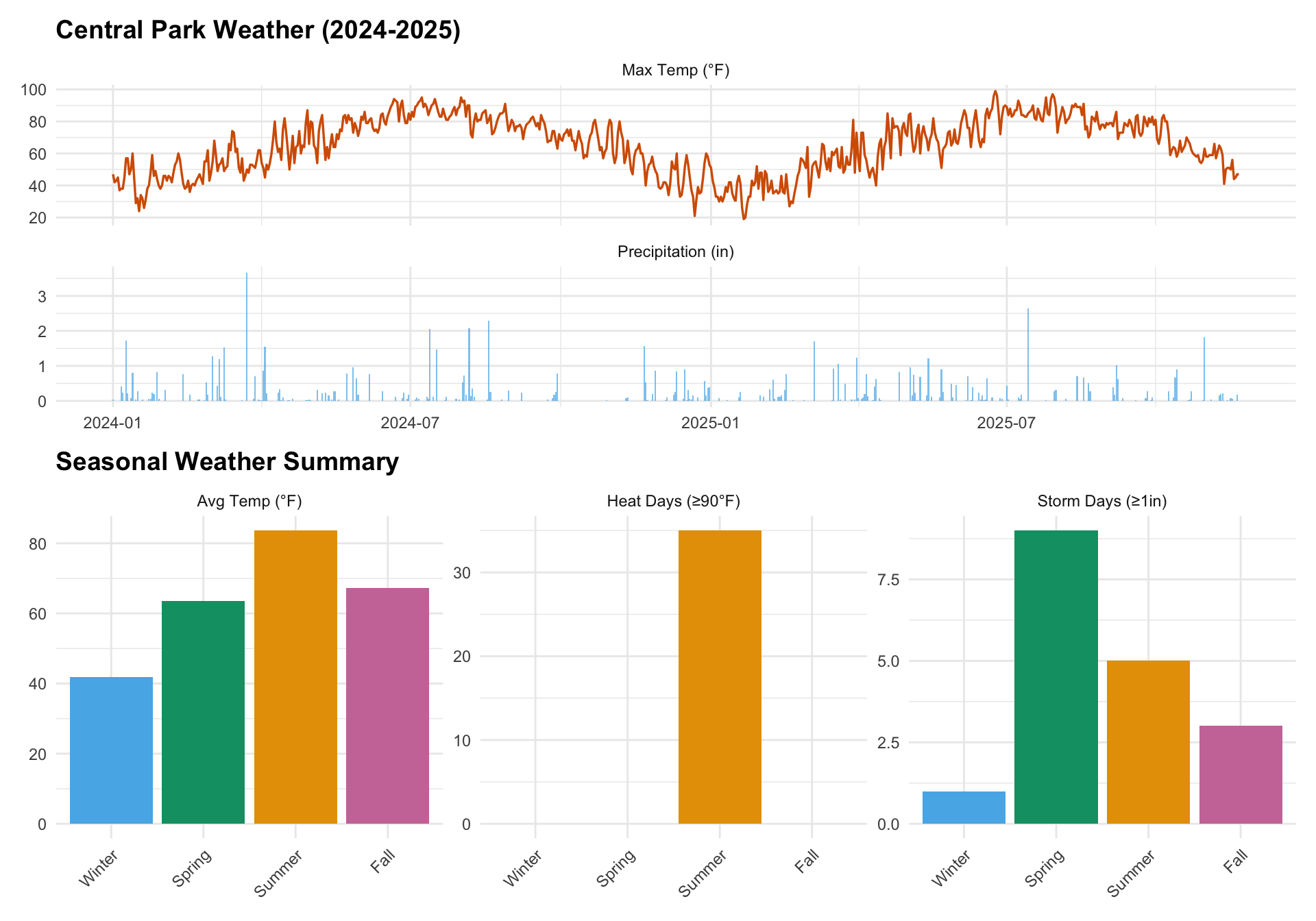

Key observations:

Temperature follows expected seasonal patterns with summer highs reaching 90°F+ and winter lows near freezing. The daily variation is substantial (20-30°F swings common), creating natural experiments for studying temperature effects on ridership.
Precipitation is episodic rather than seasonal—significant rain events (≥1 inch) occur year-round but cluster in spring and fall. These storm days represent potential ridership disruptions.
Seasonal summary confirms summer has the most heat days (≥90°F) while storm days distribute across spring, summer, and fall. Winter shows fewer extreme events but presents its own challenges (snow, cold).

Download script: download_noaa_weather.R

Permitted Events

The NYC Permitted Event Information - Historical dataset (bkfu-528j) contains comprehensive event records but includes hundreds of thousands of small-scale activities (youth sports, film shoots, farmers markets) unlikely to significantly impact subway ridership.

Smart Filtering Strategy:

Since the dataset lacks attendance information, we filtered for large events (likely 100+ people) using event characteristics as proxies:

Event types: Parades, Athletic Races/Tours, Street Events, Block Parties, Sidewalk Sales
Street impact: Events requiring full street closures
Exclusions: Youth/adult sports leagues, production events, small farmers markets

This filtering reduced from ~2 million total events to 149,524 large events across NYC.

events <- read_csv('data/events/nyc_large_events_2024_2025.csv', show_col_types = FALSE) |>
  mutate(start_date = as.Date(start_date_time), end_date = as.Date(end_date_time))

events_analysis <- events |>
  filter(!is.na(start_date)) |>
  mutate(
    month = month(start_date, label = TRUE),
    year_month = format(start_date, "%Y-%m"),
    borough = case_when(
      str_detect(tolower(event_borough), "manhattan") ~ "Manhattan",
      str_detect(tolower(event_borough), "brooklyn") ~ "Brooklyn",
      str_detect(tolower(event_borough), "queens") ~ "Queens",
      str_detect(tolower(event_borough), "bronx") ~ "The Bronx",
      str_detect(tolower(event_borough), "staten island") ~ "Staten Island",
      TRUE ~ "Other"
    )
  )

Successfully downloaded 149,524 large events (Jan 2024 - Oct 2025), including 53,977 in Manhattan.

# Monthly time series by borough
p_events_time <- events_analysis |>
  count(year_month, borough) |>
  mutate(date = as.Date(paste0(year_month, "-01"))) |>
  ggplot(aes(x = date, y = n, fill = borough)) +
  geom_col() +
  scale_fill_manual(values = c(
    "Manhattan" = okabe_ito$orange, "Brooklyn" = okabe_ito$sky_blue,
    "Queens" = okabe_ito$green, "The Bronx" = okabe_ito$vermillion,
    "Staten Island" = okabe_ito$pink, "Other" = "#999999"
  )) +
  scale_x_date(date_labels = "%b %Y", date_breaks = "3 months") +
  labs(title = "Large NYC Events by Borough (2024-2025)",
       subtitle = "Strong seasonal pattern: summer/fall peaks, winter lows",
       x = NULL, y = "Number of Events", fill = "Borough") +
  theme(axis.text.x = element_text(angle = 45, hjust = 1), legend.position = "right")

# Top event types in Manhattan
p_event_types <- events_analysis |>
  filter(borough == "Manhattan", !is.na(event_type)) |>
  count(event_type, sort = TRUE) |>
  slice_max(n, n = 8) |>
  mutate(event_type = fct_reorder(event_type, n)) |>
  ggplot(aes(x = n, y = event_type)) +
  geom_col(fill = "#F77F00") +
  scale_x_continuous(labels = comma) +
  labs(title = "Top Event Types in Manhattan", x = "Number of Events", y = NULL) +
  theme(plot.title = element_text(size = 11))

p_events_time / p_event_types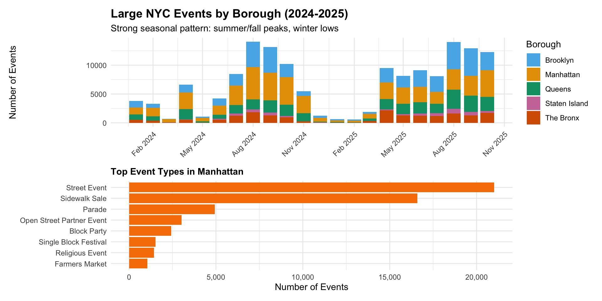

Key observations:

Monthly distribution reveals strong seasonality—event counts peak in summer and early fall (June-October) when outdoor activities flourish, then drop sharply in winter months. Manhattan consistently hosts the largest share of citywide events.
Event types in Manhattan are dominated by street events (street fairs, festivals) and block parties, followed by athletic events (marathons, races). Parades, while fewer in number, often represent the largest individual events (NYC Marathon, Pride March, etc.).
Borough comparison shows Manhattan’s event density far exceeds other boroughs, reflecting its role as NYC’s commercial and cultural center—important context for our station-level impact analysis.

Download script: download_historical_events_monthly.R

Station Locations

Station coordinates are already embedded in the ridership data, so we extracted unique station complexes with coordinates directly from the ridership API rather than seeking a separate geospatial dataset.

stations <- read_csv('data/stations/mta_station_complexes.csv', show_col_types = FALSE) |>
  distinct(station_complex_id, .keep_all = TRUE)
manhattan_stations <- stations |>
  filter(borough == "Manhattan", !is.na(latitude), !is.na(longitude))

We identified 427 unique station complexes across NYC, with 123 in Manhattan covering the entire borough from Battery Park to Inwood.

library(sf)

# Calculate total ridership by station
station_ridership <- ridership |>
  group_by(station_complex_id, station_complex) |>
  summarize(total_ridership = sum(total_ridership, na.rm = TRUE) / 1e6, .groups = "drop")

# Join with station coordinates
manhattan_stations_ridership <- manhattan_stations |>
  left_join(station_ridership, by = c("station_complex_id", "station_complex")) |>
  mutate(
    longitude = as.numeric(longitude),
    latitude = as.numeric(latitude)
  ) |>
  filter(!is.na(total_ridership))

# Load NYC neighborhoods for map background
# Data preloaded by data/download_nyc_geo.R
nyc_nta <- st_read("data/geo/nyc_nta.geojson", quiet = TRUE)

# Filter to Manhattan
if ("borough" %in% names(nyc_nta)) {
  manhattan_sf <- nyc_nta %>% filter(borough == "Manhattan")
} else if ("boro_name" %in% names(nyc_nta)) {
  manhattan_sf <- nyc_nta %>% filter(boro_name == "Manhattan")
} else {
  manhattan_sf <- nyc_nta
}

# Create static map
ggplot() +
  geom_sf(data = manhattan_sf, fill = "gray92", color = "gray75", linewidth = 0.2) +
  geom_point(
    data = manhattan_stations_ridership,
    aes(x = longitude, y = latitude, color = total_ridership),
    size = 2.5,
    alpha = 0.85
  ) +
  scale_color_viridis_c(
    option = "plasma",
    name = "Total Ridership\n(Millions)",
    trans = "log10",
    labels = scales::comma
  ) +
  coord_sf(
    crs = 4326,
    xlim = c(-74.02, -73.93),
    ylim = c(40.70, 40.80)
  ) +
  labs(
    title = "Manhattan Subway Stations by Total Ridership",
    subtitle = "January 2024 - October 2025",
    x = NULL, y = NULL
  ) +
  theme_minimal() +
  theme(
    axis.text = element_blank(),
    axis.ticks = element_blank(),
    panel.grid = element_blank(),
    legend.position = "right"
  )

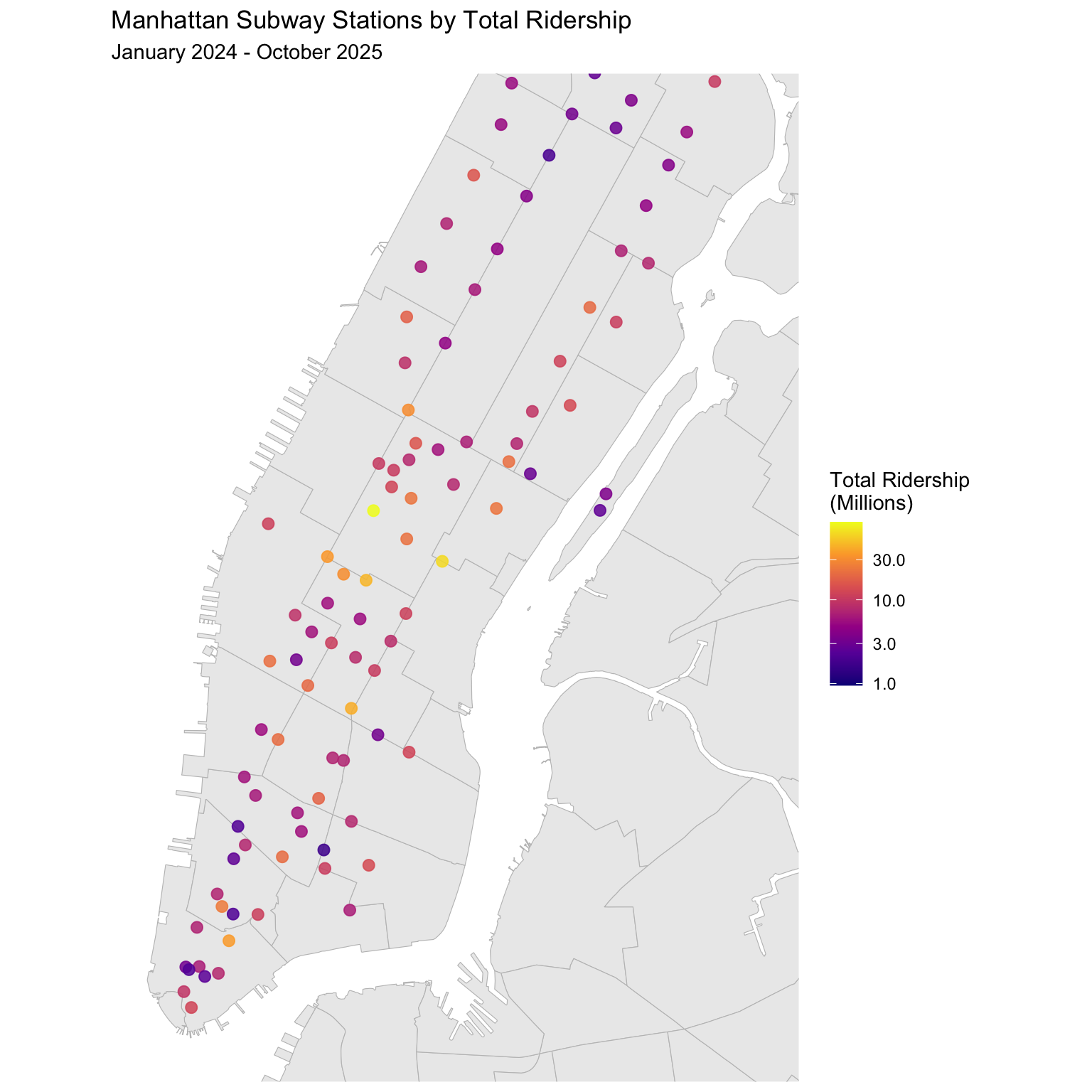
Key observations:

Spatial concentration is striking—the highest-ridership stations (bright yellow/orange) cluster in Midtown Manhattan (34th-59th Streets), forming a dense core of transit activity around Penn Station, Times Square, and Grand Central.
North-South gradient shows ridership declining as you move toward Upper Manhattan (Harlem, Washington Heights) and the Financial District edges, reflecting the concentration of employment and tourism in Midtown.
Station density varies considerably—Midtown has closely spaced stations serving office towers, while residential Upper Manhattan has wider spacing. This spatial structure influences how events and weather may differentially impact neighborhoods.

Note: Station coordinates are extracted directly from the ridership data—no separate download script required.

Part 2: Data Wrangling Pipeline

This section documents the complete data wrangling process that transforms our raw datasets into analysis-ready panels. The goal is to create a robust foundation for examining the interplay between MTA subway ridership, weather conditions, and major NYC events.

Raw Data Ingestion

We begin by loading the raw datasets and performing initial cleaning: standardizing column names, parsing date/time stamps, and filtering to Manhattan for the 2024-2025 study period.

path_rid_2024 <- "data/mta_ridership_full/ridership_2024_manhattan.csv"
path_rid_2025 <- "data/mta_ridership_full/ridership_2025_manhattan.csv"
path_weather <- "data/weather/central_park_weather_wide.csv"
path_events <- "data/events/nyc_large_events_2024_2025.csv"
path_stations <- "data/stations/mta_station_complexes.csv"

rid24 <- vroom::vroom(path_rid_2024, show_col_types = FALSE)
rid25 <- vroom::vroom(path_rid_2025, show_col_types = FALSE)
weather_raw <- readr::read_csv(path_weather, show_col_types = FALSE)
events_raw <- vroom::vroom(path_events, show_col_types = FALSE)
stations_raw <- readr::read_csv(path_stations, show_col_types = FALSE)

rid <- bind_rows(rid24, rid25) |>
  clean_names() |>
  mutate(
    # Handle both datetime and date-only formats
    transit_timestamp = parse_date_time(transit_timestamp, orders = c("ymd HMS", "ymd"), quiet = TRUE),
    date = as_date(transit_timestamp),
    hour = hour(transit_timestamp)
  ) |>
  select(station_complex_id, station_complex, borough, transit_timestamp, date, hour, total_ridership)

weather_clean <- weather_raw |>
  clean_names() |>
  mutate(
    date = as_date(date),
    tmax = as.numeric(tmax),
    prcp = as.numeric(prcp),
    snow = as.numeric(snow)
  ) |>
  select(date, tmax, prcp, snow) |>
  arrange(date)

events_clean <- events_raw |>
  clean_names() |>
  mutate(
    start_dt = ymd_hms(start_date_time, quiet = TRUE),
    end_dt = ymd_hms(end_date_time, quiet = TRUE),
    event_borough = str_to_lower(event_borough)
  ) |>
  filter(!is.na(start_dt), !is.na(end_dt), end_dt >= start_dt)

stations_clean <- stations_raw |>
  clean_names() |>
  filter(str_to_lower(borough) == "manhattan", !is.na(latitude), !is.na(longitude))

Station-Hour Panel Construction

The most granular unit of our analysis is the station-hour. We build the primary panel_station_hour dataset and calculate hours_present per station-day to identify potential missing data.

panel_station_hour <- rid |>
  select(station_complex_id, station_complex, date, hour, total_ridership) |>
  arrange(station_complex_id, date, hour)

hour_cov <- panel_station_hour |>
  group_by(station_complex_id, date) |>
  summarize(hours_present = n_distinct(hour), .groups = "drop")

Station-Day Aggregation

For analyses focusing on daily impacts (e.g., heatwaves), we aggregate to panel_station_day by summing total ridership for each station on each day.

panel_station_day <- panel_station_hour |>
  group_by(station_complex_id, station_complex, date) |>
  summarize(
    entries_day = sum(total_ridership, na.rm = TRUE),
    .groups = "drop"
  ) |>
  left_join(hour_cov, by = c("station_complex_id", "date")) |>
  mutate(hours_present = replace_na(hours_present, 0L))

Weather Feature Engineering

We integrate daily weather observations and engineer two key features:

heatwave: Binary indicator for periods with max temperature ≥ 90°F for consecutive days
storm: Binary indicator for significant precipitation events (≥ 1 inch)

panel_station_day <- panel_station_day |>
  left_join(weather_clean, by = "date") |>
  arrange(station_complex_id, date) |>
  group_by(station_complex_id) |>
  mutate(
    heat_day = if_else(!is.na(tmax) & tmax >= params$heat_threshold_f, 1L, 0L),
    heat_roll = slide_int(heat_day, sum, .before = params$heat_consec_days - 1, .complete = TRUE),
    heatwave = if_else(!is.na(heat_roll) & heat_roll >= params$heat_consec_days, 1L, 0L),
    storm = if_else(!is.na(prcp) & prcp >= params$storm_threshold_in, 1L, 0L),
    weather_missing = as.integer(is.na(tmax) | is.na(prcp))
  ) |>
  ungroup()

Event Geocoding & Spatial Matching

This critical step links textual event data to subway stations:

Filter to large-scale Manhattan events (parades, races, festivals)
Geocode text addresses to coordinates using ArcGIS/OSM
Spatial join events to nearest station within 800m radius
Flag affected station-hours and station-days

event_radius_m <- params$event_radius_m

# Filter to Manhattan focus events
events_manhattan <- events_clean |>
  filter(is.na(event_borough) | str_detect(event_borough, "manhattan"))

focus_types <- c("parade", "athletic", "race", "tour", "street", "block", "festival", "fair")
events_focus <- events_manhattan |>
  filter(!is.na(event_type)) |>
  filter(purrr::reduce(focus_types, \(acc, key) acc | str_detect(str_to_lower(event_type), key), .init = FALSE)) |>
  distinct(event_id, .keep_all = TRUE) |>
  mutate(event_id = as.character(event_id))

# Load geocode cache
cache_path <- "data/events/nyc_large_events_geocoded.csv"
if (file.exists(cache_path)) {
  geo_cache <- readr::read_csv(
    cache_path,
    col_types = cols(.default = col_guess(), event_id = col_character()),
    show_col_types = FALSE
  )
} else {
  geo_cache <- tibble(event_id = character(), lon = numeric(), lat = numeric())
}

# Join with geocoded coordinates
events_focus_geo <- events_focus |>
  left_join(geo_cache, by = "event_id")

evt_geo_ok <- events_focus_geo |>
  filter(!is.na(lon), !is.na(lat)) |>
  mutate(
    start_hr = floor_date(start_dt, "hour"),
    end_hr = ceiling_date(end_dt, "hour")
  )

# Spatial matching to stations
if (nrow(evt_geo_ok) == 0) {
  events_station_hour <- tibble(
    station_complex_id = character(),
    date = as.Date(character()),
    hour = integer(),
    event_hour = integer()
  )
} else {
  stn_sf <- st_as_sf(stations_clean, coords = c("longitude", "latitude"), crs = 4326) |>
    st_transform(2263)
  evt_sf <- st_as_sf(evt_geo_ok, coords = c("lon", "lat"), crs = 4326) |>
    st_transform(2263)

  near_idx <- st_nearest_feature(evt_sf, stn_sf)
  dist_ft <- st_distance(evt_sf, stn_sf[near_idx, ], by_element = TRUE)
  dist_m <- as.numeric(dist_ft) * 0.3048

  evt_joined <- evt_geo_ok |>
    mutate(
      station_complex_id = stn_sf$station_complex_id[near_idx],
      dist_m = dist_m
    ) |>
    filter(dist_m <= event_radius_m) |>
    select(event_id, station_complex_id, start_hr, end_hr, dist_m)

  events_station_hour <- purrr::map_dfr(seq_len(nrow(evt_joined)), function(i) {
    tibble(
      station_complex_id = evt_joined$station_complex_id[i],
      hour_ts = seq(evt_joined$start_hr[i], evt_joined$end_hr[i], by = "1 hour")
    )
  }) |>
    mutate(date = as_date(hour_ts), hour = hour(hour_ts), event_hour = 1L) |>
    distinct(station_complex_id, date, hour, .keep_all = TRUE) |>
    select(station_complex_id, date, hour, event_hour)
}

# Join events to panels
panel_station_hour <- panel_station_hour |>
  left_join(events_station_hour, by = c("station_complex_id", "date", "hour")) |>
  mutate(event_hour = if_else(is.na(event_hour), 0L, event_hour))

event_day_by_station <- panel_station_hour |>
  group_by(station_complex_id, date) |>
  summarize(event_day = as.integer(any(event_hour == 1L)), .groups = "drop")

panel_station_day <- panel_station_day |>
  left_join(event_day_by_station, by = c("station_complex_id", "date")) |>
  mutate(event_day = if_else(is.na(event_day), 0L, event_day))

Holiday Flags

We flag US federal holidays using the timeDate package, as ridership patterns on holidays often mimic Sunday schedules.

holidays <- tibble(
  date = as.Date(holidayNYSE(2024:2025)),
  is_holiday = "Yes"
)

panel_station_day <- panel_station_day |>
  left_join(holidays, by = "date") |>
  mutate(
    is_holiday = case_match(
      is_holiday,
      NA ~ "No",
      "Yes" ~ "Yes"
    )
  )

Baseline Calculation

To calculate percent change in ridership, we define the baseline as the median ridership for each station by day-of-week and month, accounting for weekly and seasonal patterns.

panel_station_day <- panel_station_day |>
  mutate(
    dow = wday(date, label = TRUE, week_start = 1),
    month = month(date)
  )

baseline_sd <- panel_station_day |>
  group_by(station_complex_id, dow, month) |>
  summarize(baseline_sd = median(entries_day, na.rm = TRUE), .groups = "drop")

panel_station_day <- panel_station_day |>
  left_join(baseline_sd, by = c("station_complex_id", "dow", "month")) |>
  mutate(
    pct_change = log((entries_day + 1) / (baseline_sd + 1))
  )

baseline_sh <- panel_station_hour |>
  mutate(
    dow = wday(date, label = TRUE, week_start = 1),
    month = month(date)
  ) |>
  group_by(station_complex_id, dow, month, hour) |>
  summarize(baseline_sh = median(total_ridership, na.rm = TRUE), .groups = "drop")

panel_station_hour <- panel_station_hour |>
  mutate(
    dow = wday(date, label = TRUE, week_start = 1),
    month = month(date)
  ) |>
  left_join(baseline_sh, by = c("station_complex_id", "dow", "month", "hour")) |>
  mutate(
    hourly_pct_change = log((total_ridership + 1) / (baseline_sh + 1))
  )

Output Summary

cat("Panel Station Day:", nrow(panel_station_day), "rows\n")

## Panel Station Day: 80905 rows

cat("Panel Station Hour:", nrow(panel_station_hour), "rows\n")

## Panel Station Hour: 1921163 rows

cat("Stations:", n_distinct(panel_station_day$station_complex_id), "\n")

## Stations: 123

cat("Date range:", as.character(min(panel_station_day$date, na.rm = TRUE)), "to", as.character(max(panel_station_day$date, na.rm = TRUE)), "\n")

## Date range: 2024-01-01 to 2025-10-19

cat("Heatwave days:", sum(panel_station_day$heatwave == 1, na.rm = TRUE), "\n")

## Heatwave days: 1108

cat("Storm days:", sum(panel_station_day$storm == 1, na.rm = TRUE), "\n")

## Storm days: 2090

cat("Event-affected station-days:", sum(panel_station_day$event_day == 1, na.rm = TRUE), "\n")

## Event-affected station-days: 2504

if (params$write_outputs) {
  write_parquet(panel_station_day, file.path(params$outputs_dir, "panel_station_day_indexed.parquet"))
  write_parquet(panel_station_hour, file.path(params$outputs_dir, "panel_station_hour_indexed.parquet"))
  cat("\nParquet files written to:", params$outputs_dir, "\n")
}

The final datasets (panel_station_day and panel_station_hour) are exported as Parquet files for efficient use in our analysis pipeline.

Data Guide

For users who want to skip the data wrangling process and jump directly into analysis, we provide pre-built Parquet files in the data/derived/ directory. These files contain the fully processed panel datasets ready for modeling and visualization.

Quick Start

To load the prepared datasets, simply run:

library(arrow)

# Load the station-day panel (recommended for most analyses)
panel_day <- read_parquet("data/derived/panel_station_day_indexed.parquet")

# Load the station-hour panel (for hourly/intraday analyses)
panel_hour <- read_parquet("data/derived/panel_station_hour_indexed.parquet")

Available Files

File	Description	Rows	Use Case
`panel_station_day_indexed.parquet`	Station-day level ridership with weather, events, and baseline	~85K	Daily impact analysis, regression models
`panel_station_hour_indexed.parquet`	Station-hour level ridership with event flags	~2M	Hourly patterns, intraday event effects
`station_lookup.csv`	Station metadata (names, coordinates)	~120	Reference table
`station_summary.csv`	Aggregated station statistics	~120	Quick station comparisons

Key Variables

Station-Day Panel (panel_station_day_indexed.parquet):

Core identifiers:

station_complex_id: Unique station identifier
station_complex: Human-readable station name
date: Date of observation

Ridership:

entries_day: Total daily ridership at station
baseline_sd: Median ridership for this station/day-of-week/month
pct_change: Log percent change from baseline

Weather indicators:

tmax: Maximum temperature (°F)
prcp: Precipitation (inches)
snow: Snowfall (inches)
heatwave: Binary flag (1 = part of 3+ day heat spell ≥90°F)
storm: Binary flag (1 = precipitation ≥1 inch)

Event & calendar:

event_day: Binary flag (1 = nearby event active)
is_holiday: “Yes”/“No” for federal holidays
dow: Day of week (Mon-Sun)
month: Month number (1-12)

Station-Hour Panel (panel_station_hour_indexed.parquet):

Core identifiers:

station_complex_id: Unique station identifier
station_complex: Human-readable station name
date: Date of observation
hour: Hour of day (0-23)

Ridership:

total_ridership: Hourly ridership count
baseline_sh: Median ridership for this station/dow/month/hour
hourly_pct_change: Log percent change from baseline

Event flag:

event_hour: Binary flag (1 = event active during this hour)

Example Usage

Analyze heatwave impacts on ridership:

panel_station_day |>
  filter(is_holiday == "No") |>  # Exclude holidays
  group_by(heatwave) |>
  summarize(
    n_obs = n(),
    mean_ridership = mean(entries_day, na.rm = TRUE),
    mean_pct_change = mean(pct_change, na.rm = TRUE)
  )

Compare event vs. non-event hours:

panel_station_hour |>
  group_by(event_hour) |>
  summarize(
    n_obs = n(),
    mean_ridership = mean(total_ridership, na.rm = TRUE),
    mean_pct_change = mean(hourly_pct_change, na.rm = TRUE)
  )

Filter to specific stations or date ranges:

# Times Square station during summer 2024
panel_station_day |>
  filter(
    str_detect(station_complex, "Times Sq"),
    date >= "2024-06-01",
    date <= "2024-08-31"
  )

Performance Tips

Use Parquet: Parquet files load 5-10x faster than CSV and use less memory
Filter early: Apply filter() before summarize() to reduce computation
Choose the right granularity: Use station-day for most analyses; only load station-hour when hourly resolution is required

Data & Methods

Part 1: Data Sources

MTA Subway Ridership

Weather Data

Permitted Events

Station Locations

Part 2: Data Wrangling Pipeline

Raw Data Ingestion

Station-Hour Panel Construction

Station-Day Aggregation

Weather Feature Engineering

Event Geocoding & Spatial Matching

Holiday Flags

Baseline Calculation

Output Summary

Data Guide

Quick Start

Available Files

Key Variables

Example Usage

Performance Tips